Dealing with uncertainty: sensitivity analysis

3. Dealing with uncertainty: sensitivity analysis#

3.1. Uncertainty#

It is important that we do not just set up our model, pick values for our parameters, run our model and look at the results, and then call it a day. We need to consider uncertainty in our work.

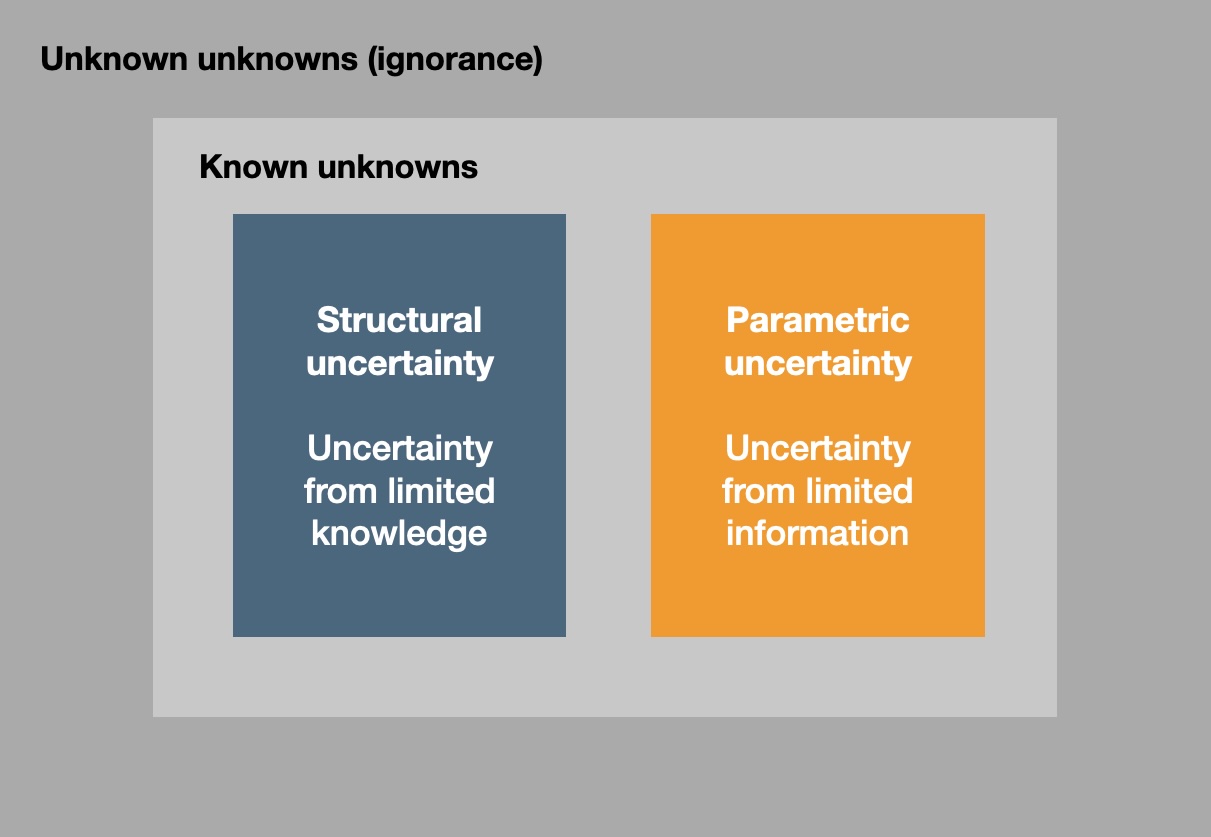
../_images/uncertainty-types.jpg — Fig. 3.1 Different kinds of uncertainty. Based on a talk by David Spiegelhalter, “Uncertainty in Decision Models” (not available online).#

There are many ways in which people have classified uncertainty. Here we want to distinguish between structural and parametric uncertainty (Figure Fig. 3.1). You could say that structural uncertainty arises from how the model is set up. It deals with the limitations or assumptions made about the system being modelled. For instance, assuming a linear relationship in a system that is actually non-linear is a structural issue in our model. Dealing with structural uncertainty can be quite challenging.

In contrast, parametric uncertainty relates to the parameters used in the model: the numbers we fill in. Ignoring whether or not the structure of the model is adequate, are we confident about our input data? How uncertain are our parameters?

This is where sensitivity analysis comes in.

3.2. Sensitivity in the economic dispatch example#

We want to use sensitivity analysis to investigate how the optimal solution to an optimisation problem changes if we change some parameters in the problem, for example, the coefficients in the objective function or constraints. To illustrate this, we will revisit the economic dispatch problem from Section 2.1. Recall the problem is:

(3.1)#\[\begin{align} \text{Min.} \; & J = 3P_1 + 4P_2 \\ \text{s.t.} \; & 50 \leq P_1 \leq 300 \\ & 100 \leq P_2 \leq 400 \\ & P_1 + P_2 = 500 \\ \end{align}\]

3.2.1. Changing objective function coefficients#

For example, we can change the objective function so that it reads \(J = 5P_1 + 4P_2\). The result of this is easy to work out: Now, \(P_1\) is more expensive than \(P_2\), so we will flip to the second of the two possible solutions (see Figure Fig. 2.5).

What is important to realise is that changing the objective function does not change the shape of the feasible region in any way. The feasible region’s shape and boundaries stay fixed, but the point that represents the optimal solution may move to a different location within the region.

3.2.2. Changing constraint parameters#

Recall that some constraints are active: they are actively “fencing us in” and pushing us to our current optimal solution. In our current example, one such active constraint is the generation capacity of the coal plant (\(P_1\)), which is limited to a maximum of 300 MW. In our optimal solution, we are at this boundary: \(P_1 = 300\).

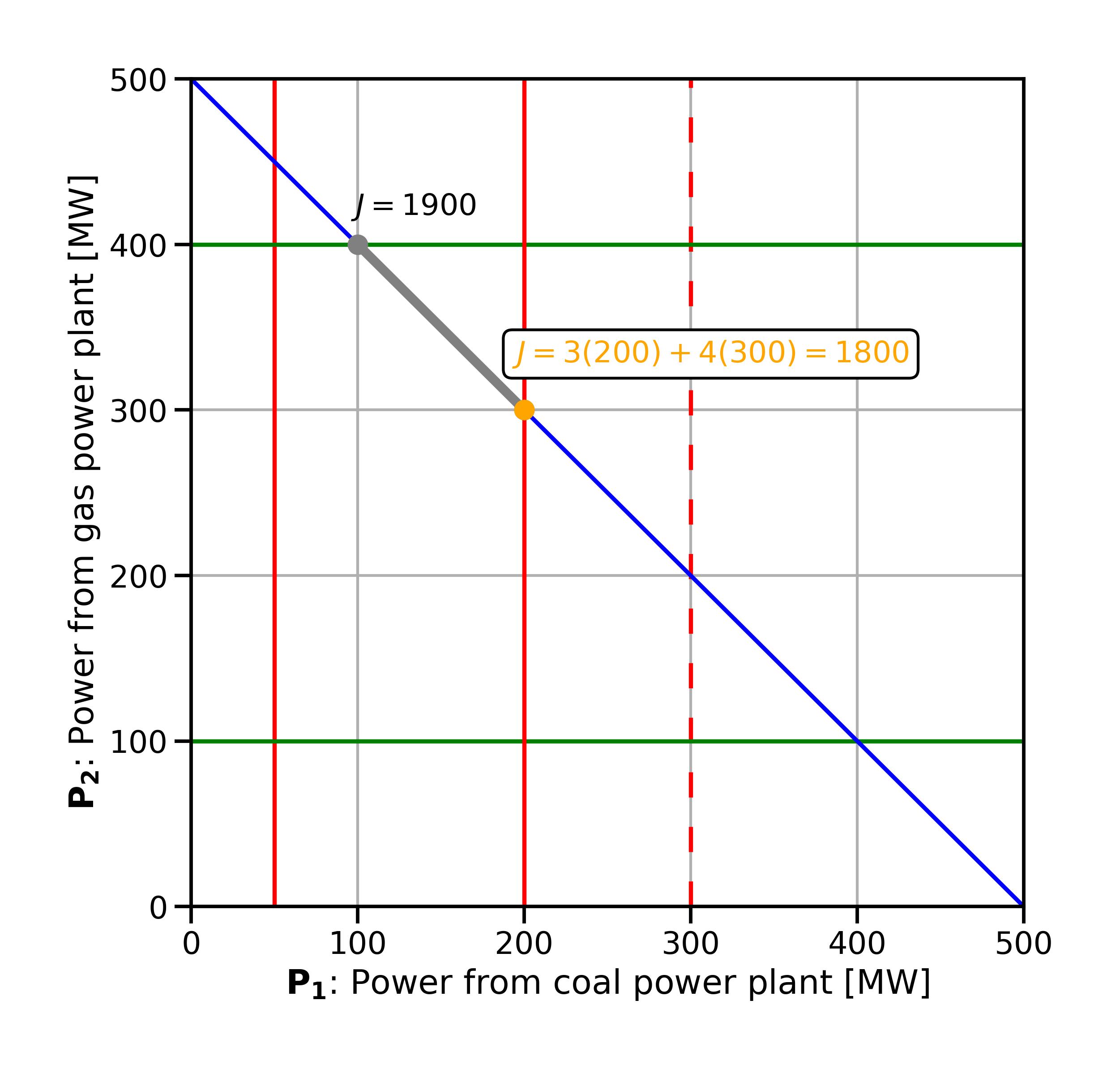
Now, we will change the constraint on \(P_1\): \(50 \leq P_1 \leq 200\). This changes the shape of the decision space, as seen in Fig. 3.2. As a result, the optimal solution also changes, with \(P_1^* = 200\), \(P_2^* = 300\), and \(J = 1800\).

../_images/fig_sensitivitylp_changed_plantconstraint.jpg — Fig. 3.2 Effect of changing the constraint parameter for power plant (unit) 1.#

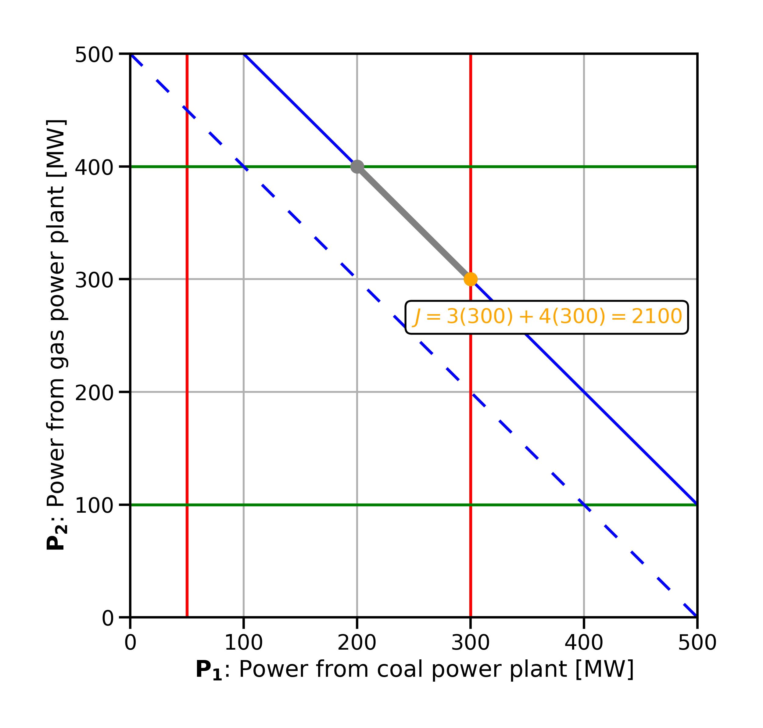
Now let’s go back to the original economic dispatch problem and change a different constraint. This time we change the demand constraint to \(P_1 + P_2 = 600\). The feasible region again changes: the demand increased so the demand constraint (equality constraint) line is shifted in Fig. 3.3. We get a new optimal solution: \(P_1^* = 300\), \(P_2^* = 300\), and \(J = 2100\).

../_images/fig_sensitivitylp_changed_demandconstraint.jpg — Fig. 3.3 Effect of changing the demand constraint.#

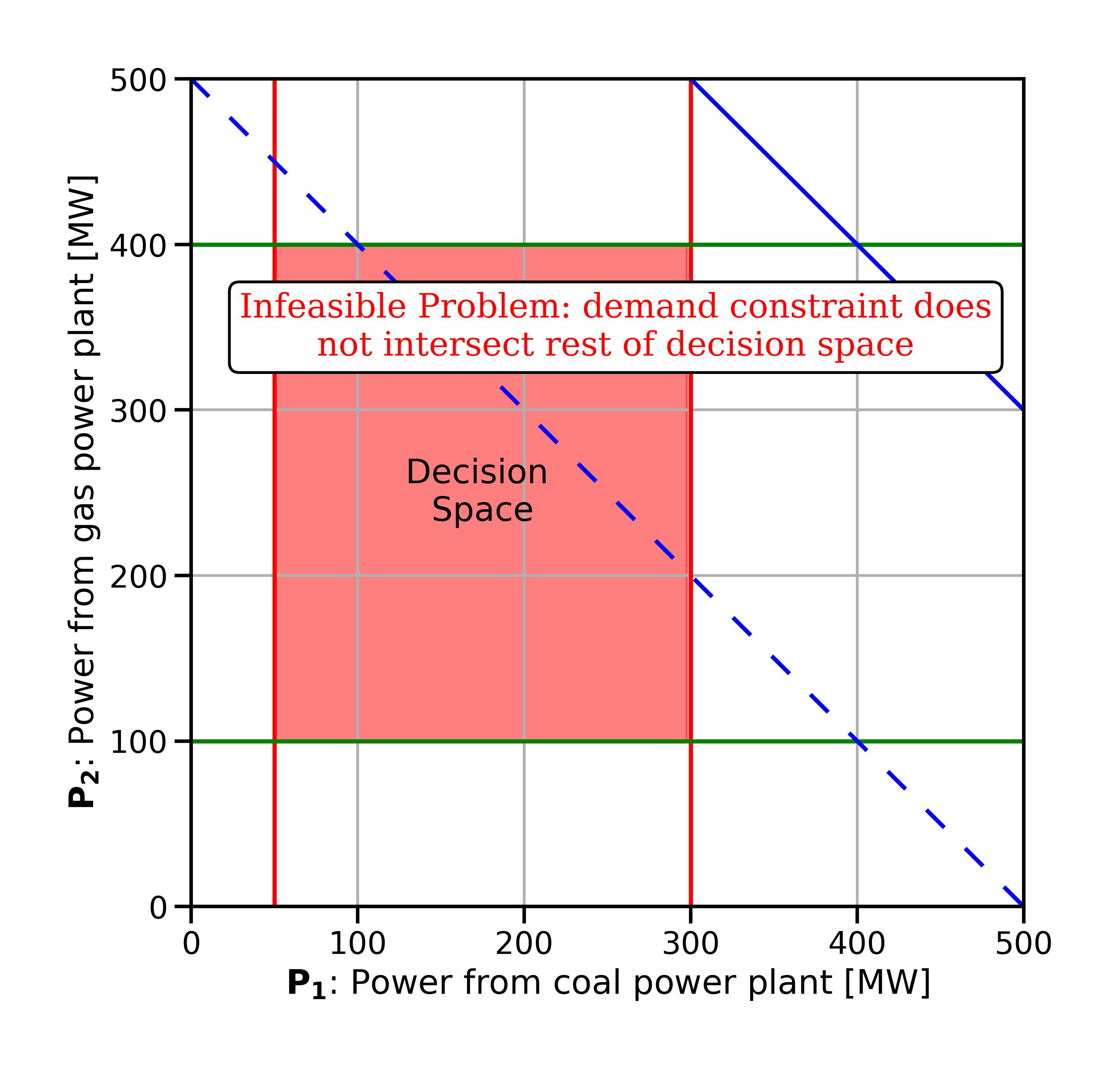
What if we increase the power demand even more, say to 800? So \(P_1 + P_2 = 800\). Now an interesing situation arises. If we look at Fig. 3.4, we can see that now we actually have an infeasible problem. This is because the operational constraints on units 1 and 2 do not intersect with the new demand constraint. There is no possible feasible solution.

../_images/fig_sensitivitylp_changed_demandconstraint_infeasible.jpg — Fig. 3.4 Changing the demand constraint to such a high value that the problem becomes infeasible.#

3.3. Shadow prices: effect of changing active constraints#

As a part of sensitivity analysis, we want to calculate the effect that changing a parameter in an active constraint has on the optimal solution (non-active constraints have no effect on the solution, since they are not constraining us at the moment). To do so we can analyse small changes of the parameters.

Returning to the economic dispatch example, the active constraints are \(P_1 \leq 300\) and \(P_1 + P_2 = 500\). First we’ll analyse the sensitivity of the maximum generation capacity constraint on unit 1: \(P_1 \leq 300\). To do this, we change the constraint parameter by \(+1\) so \(P_1 \leq 301\). Then we solve the new optimisation problem. We find that the new objective function value is \(J = 1699\). Compared to the original objective function value, \(J = 1700\), this is 1 less. Therefore, we can say that changing the right-hand side of the coal plant constraint by +1 changes the optimal solution by -1.

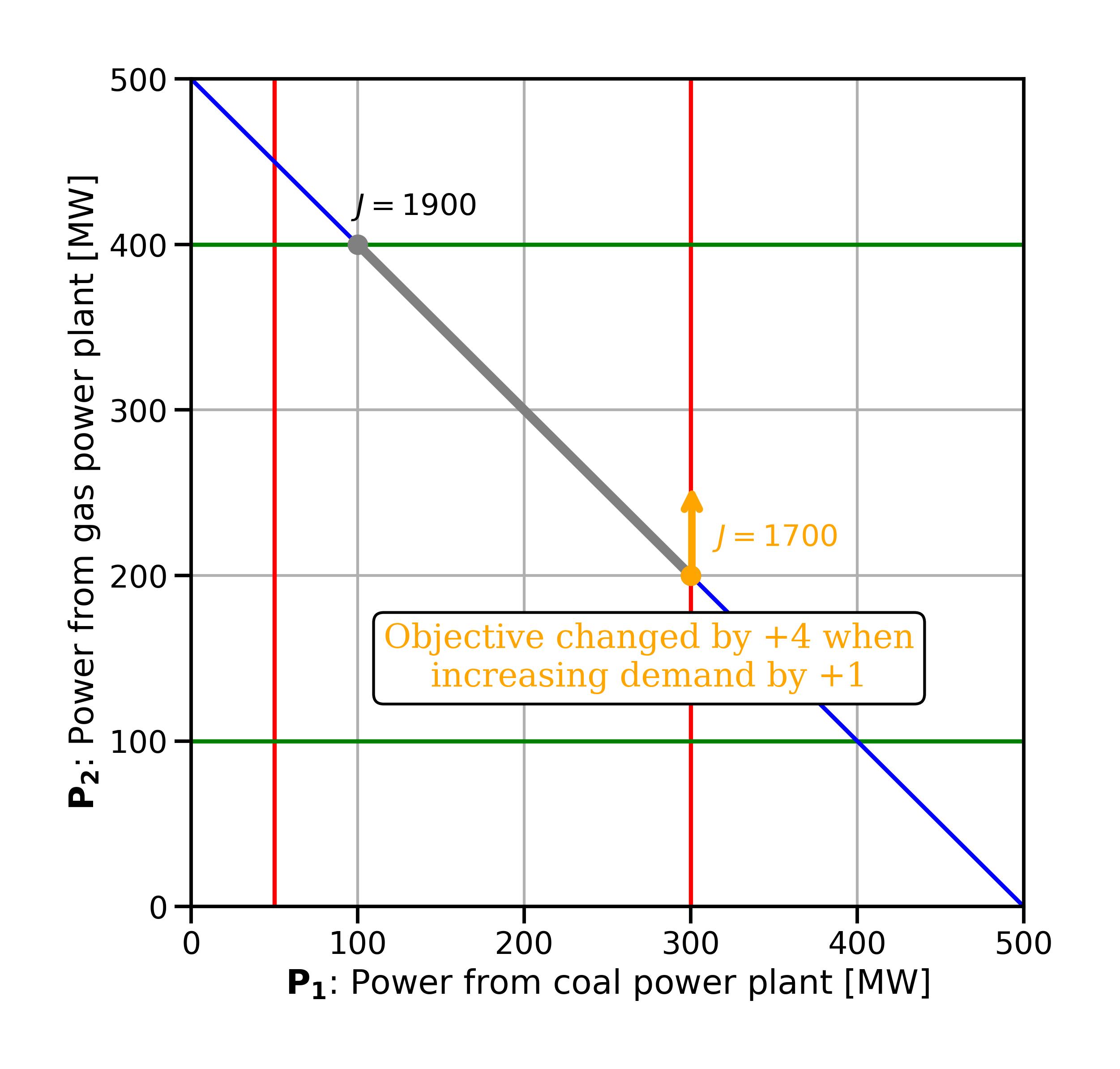
Next let’s analyse the other active constraint, the demand constraint. We change it to \(P_1 + P_2 = 501\) and re-solve the optimisation problem. The result is \(J = 1704\). So, changing the right-hand side of the demand constraint by +1 changes the optimal solution by +4. See this in Fig. 3.5.

../_images/fig_sensitivitylp_shadowprice.jpg — Fig. 3.5 Changing the demand by +1 changes the optimal solution by +4; the shadow price of the power demand is +4#

These changes that we just observed are called shadow prices. The shadow price is the change in the optimal objective value if the right-hand side of an active constraint increases by a marginal amount. All other parts of the problem remain unchanged. The shadow price is the marginal cost or marginal benefit of relaxing a certain constraint. In the case of the demand constraint (\(P_1 + P_2 = 500\)), we can interpret the shadow price as the marginal cost of supplying an additional unit of demand.

It is important to note that only active constraints affect the objective function value in the optimal solution. Therefore, inactive constraints have a shadow price of zero. The shadow price is concerned only with marginal changes, and inactive constraints do not contribute to these changes.

Infinitesimally small changes

Above, we manually changed the parameters in our constraints by +1 to see - again manually - the effect on the objective function. This helps understand what is happening as we relax a constraint. Formally, however, the shadow price represents an infinitesimally small change. You could interpret it as the derivative of the objective function with respect to the specific constraint being relaxed. If the change becomes too large, the structure of the problem will change: new constraints become active and old ones might become inactive. That’s not what we want to do here - we want to look at changed within an “allowable range” that doesn’t change the problem. Hence, we are strictly speaking only looking at infinitesimally small changes.

In section Section 4.1, we will introduce the concept of duality - and see how thanks to duality, we can obtain the shadow prices of a linear optimisation problem easily and automatically, without any manual fiddling of the type we did above.